Working_With_Time_Series
Working_With_Time_Series
시계열 다루기 Working_With_Time_Series
타임 스탬프 : 특정 시점을 말함
시간 간격 : 특정 시작점과 종료점 사이의 시간의 길이
기간 : 일반적으로 각 간격이 일정하고 서로 곂치지 않는 특별한 경우의 시간 간격
시간 델타, 지속 기간 : 정확한 시간 길이
Dates and Times in Python
Native Python dates and times: datetime and dateutil
1
2
3
4
from datetime import datetime

# 날짜를 직접 구성
datetime(year=2015, month=7, day=4)
1
datetime.datetime(2015, 7, 4, 0, 0)
1
2
3
4
5
from dateutil import parser

# 다양한 문자열 형태로부터 날짜를 해석
date = parser.parse("4th of July, 2015")
date
1
datetime.datetime(2015, 7, 4, 0, 0)
1
2
# 요일을 출력
date.strftime('%A')
1
'Saturday'
Typed arrays of times: NumPy’s datetime64
1
2
3
4
5
import numpy as np

# datetime64 dtype은 날짜를 64비트 정수로 인코딩
date = np.array('2015-07-04', dtype=np.datetime64)
date
1
array('2015-07-04', dtype='datetime64[D]')
1
2
# 벡터화 연산 가능
date + np.arange(12)
1
2
3
4
array(['2015-07-04', '2015-07-05', '2015-07-06', '2015-07-07',
       '2015-07-08', '2015-07-09', '2015-07-10', '2015-07-11',
       '2015-07-12', '2015-07-13', '2015-07-14', '2015-07-15'],
      dtype='datetime64[D]')
1
2
# 하루 단위
np.datetime64('2015-07-04')
1
numpy.datetime64('2015-07-04')
1
2
# 분 단위
np.datetime64('2015-07-04 12:00')
1
numpy.datetime64('2015-07-04T12:00')
1
2
# 시간 단위 --> 나노초
np.datetime64('2015-07-04 12:59:59.50', 'ns')
1
numpy.datetime64('2015-07-04T12:59:59.500000000')
날짜와 시간 코드
| Code | Meaning | Time span (relative) | Time span (absolute) |
|---|---|---|---|
Y | Year | ± 9.2e18 years | [9.2e18 BC, 9.2e18 AD] |
M | Month | ± 7.6e17 years | [7.6e17 BC, 7.6e17 AD] |
W | Week | ± 1.7e17 years | [1.7e17 BC, 1.7e17 AD] |
D | Day | ± 2.5e16 years | [2.5e16 BC, 2.5e16 AD] |
h | Hour | ± 1.0e15 years | [1.0e15 BC, 1.0e15 AD] |
m | Minute | ± 1.7e13 years | [1.7e13 BC, 1.7e13 AD] |
s | Second | ± 2.9e12 years | [ 2.9e9 BC, 2.9e9 AD] |
ms | Millisecond | ± 2.9e9 years | [ 2.9e6 BC, 2.9e6 AD] |
us | Microsecond | ± 2.9e6 years | [290301 BC, 294241 AD] |
ns | Nanosecond | ± 292 years | [ 1678 AD, 2262 AD] |
ps | Picosecond | ± 106 days | [ 1969 AD, 1970 AD] |
fs | Femtosecond | ± 2.6 hours | [ 1969 AD, 1970 AD] |
as | Attosecond | ± 9.2 seconds | [ 1969 AD, 1970 AD] |
Dates and times in pandas: best of both worlds
1
2
3
4
import pandas as pd

date = pd.to_datetime("4th of July, 2015")
date
1
Timestamp('2015-07-04 00:00:00')
1
date.strftime('%A')
1
'Saturday'
1
2
# NumPy 스타일 벡터화 연산
date + pd.to_timedelta(np.arange(12), 'D')
1
2
3
4
DatetimeIndex(['2015-07-04', '2015-07-05', '2015-07-06', '2015-07-07',
               '2015-07-08', '2015-07-09', '2015-07-10', '2015-07-11',
               '2015-07-12', '2015-07-13', '2015-07-14', '2015-07-15'],
              dtype='datetime64[ns]', freq=None)
Pandas Time Series: Indexing by Time
1
2
3
4
5
# 시간 인덱스를 가진 데이터의 Series 객체 구성
index = pd.DatetimeIndex(['2014-07-04', '2014-08-04',
                          '2015-07-04', '2015-08-04'])
data = pd.Series([0, 1, 2, 3], index=index)
data
1
2
3
4
5
2014-07-04    0
2014-08-04    1
2015-07-04    2
2015-08-04    3
dtype: int64
1
2
# Series 인덱싱 패턴
data['2014-07-04':'2015-07-04']
1
2
3
4
2014-07-04    0
2014-08-04    1
2015-07-04    2
dtype: int64
1
2
# 인덱싱 연산
data['2015']
1
2
3
2015-07-04    2
2015-08-04    3
dtype: int64
Pandas Time Series Data Structures
타임스탬프 : numpy.datetime64 데이터 타입 기반 –> 관련 인덱스 구조 : DatetimeIndex
기간(time period) : numpy.datetime64 기반, 고정 주파수 간격을 인코딩 –> 관련 인덱스 구조 : PeriodIndex
시간 델타, 지속 기간 : datetime.timedelta 타입의 효율적 대체 타입, numpy.timedelta64 기반 –> 관련 인덱스 구조 : TimedeltaIndex
1
2
3
4
# 단일 날짜를 pd.to_datetime()에 전달하면 TimeStamp 생성하고, 일련의 날짜를 전달하면 DatetimeIndex를 생성
dates = pd.to_datetime([datetime(2015, 7, 3), '4th of July, 2015',
                        '2015-Jul-6', '07-07-2015', '20150708'])
dates
1
2
3
DatetimeIndex(['2015-07-03', '2015-07-04', '2015-07-06', '2015-07-07',
               '2015-07-08'],
              dtype='datetime64[ns]', freq=None)
1
2
# 주기(frequency) 코드를 추가해 PeriodIndex로 전환
dates.to_period('D')
1
2
3
PeriodIndex(['2015-07-03', '2015-07-04', '2015-07-06', '2015-07-07',
             '2015-07-08'],
            dtype='period[D]')
1
2
# TimedeltaIndex 생성
dates - dates[0]
1
TimedeltaIndex(['0 days', '1 days', '3 days', '4 days', '5 days'], dtype='timedelta64[ns]', freq=None)
Regular sequences: pd.date_range()
1
2
# 시작일, 종료일, 선택적 주기 코드를 받아 정규 날짜 시퀀스 생성
pd.date_range('2015-07-03', '2015-07-10')
1
2
3
DatetimeIndex(['2015-07-03', '2015-07-04', '2015-07-05', '2015-07-06',
               '2015-07-07', '2015-07-08', '2015-07-09', '2015-07-10'],
              dtype='datetime64[ns]', freq='D')
1
2
# 시작점과 기간의 수로 지정
pd.date_range('2015-07-03', periods=8)
1
2
3
DatetimeIndex(['2015-07-03', '2015-07-04', '2015-07-05', '2015-07-06',
               '2015-07-07', '2015-07-08', '2015-07-09', '2015-07-10'],
              dtype='datetime64[ns]', freq='D')
1
2
# freq 인수를 바꿔 간격을 조정
pd.date_range('2015-07-03', periods=8, freq='h')
1
2
3
4
5
DatetimeIndex(['2015-07-03 00:00:00', '2015-07-03 01:00:00',
               '2015-07-03 02:00:00', '2015-07-03 03:00:00',
               '2015-07-03 04:00:00', '2015-07-03 05:00:00',
               '2015-07-03 06:00:00', '2015-07-03 07:00:00'],
              dtype='datetime64[ns]', freq='h')
1
2
# 기간이나 타임 델타값의 정규 시퀀스 생성
pd.period_range('2015-07', periods=8, freq='M')
1
2
3
PeriodIndex(['2015-07', '2015-08', '2015-09', '2015-10', '2015-11', '2015-12',
             '2016-01', '2016-02'],
            dtype='period[M]')
1
2
# 시간단위로 증가하는 기간의 시퀀스 생성
pd.timedelta_range(0, periods=10, freq='h')
1
2
3
4
5
TimedeltaIndex(['0 days 00:00:00', '0 days 01:00:00', '0 days 02:00:00',
                '0 days 03:00:00', '0 days 04:00:00', '0 days 05:00:00',
                '0 days 06:00:00', '0 days 07:00:00', '0 days 08:00:00',
                '0 days 09:00:00'],
               dtype='timedelta64[ns]', freq='h')
Frequencies and Offsets
Pandas 주기 코드
| Code | Description | Code | Description |
|---|---|---|---|
D | Calendar day | B | Business day |
W | Weekly | ||
M | Month end | BM | Business month end |
Q | Quarter end | BQ | Business quarter end |
A | Year end | BA | Business year end |
h | Hours | BH | Business hours |
min | Minutes | ||
s | Seconds | ||
ms | Milliseonds | ||
us | Microseconds | ||
ns | nanoseconds |
주기 코드의 시작 시점을 표시하는 목록
| Code | Description | Code | Description | |
|---|---|---|---|---|
MS | Month start | BMS | Business month start | |
QS | Quarter start | BQS | Business quarter start | |
AS | Year start | BAS | Business year start |
1
2
# 코드를 숫자와 결합해 주기 지정
pd.timedelta_range(0, periods=9, freq="2h30min")
1
2
3
4
TimedeltaIndex(['0 days 00:00:00', '0 days 02:30:00', '0 days 05:00:00',
                '0 days 07:30:00', '0 days 10:00:00', '0 days 12:30:00',
                '0 days 15:00:00', '0 days 17:30:00', '0 days 20:00:00'],
               dtype='timedelta64[ns]', freq='150min')
1
2
3
4
from pandas.tseries.offsets import BDay

# 영업일 오프셋 만들기
pd.date_range('2015-07-01', periods=5, freq=BDay())
1
2
3
DatetimeIndex(['2015-07-01', '2015-07-02', '2015-07-03', '2015-07-06',
               '2015-07-07'],
              dtype='datetime64[ns]', freq='B')
Resampling, Shifting, and Windowing
1
2
3
4
5
6
7
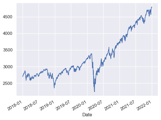
from pandas_datareader import data
import yfinance as yf
yf.pdr_override()
sp500 = data.DataReader('^GSPC', start='2018-01-01', end='2021-12-31')
sp500.head()
1
[*********************100%%**********************]  1 of 1 completed
| Open | High | Low | Close | Adj Close | Volume | |
|---|---|---|---|---|---|---|
| Date | ||||||
| 2018-01-02 | 2683.729980 | 2695.889893 | 2682.360107 | 2695.810059 | 2695.810059 | 3397430000 |
| 2018-01-03 | 2697.850098 | 2714.370117 | 2697.770020 | 2713.060059 | 2713.060059 | 3544030000 |
| 2018-01-04 | 2719.310059 | 2729.290039 | 2719.070068 | 2723.989990 | 2723.989990 | 3697340000 |
| 2018-01-05 | 2731.330078 | 2743.449951 | 2727.919922 | 2743.149902 | 2743.149902 | 3239280000 |
| 2018-01-08 | 2742.669922 | 2748.510010 | 2737.600098 | 2747.709961 | 2747.709961 | 3246160000 |
1
sp500 = sp500['Close']
1
2
3
4
5
6
7
%matplotlib
inline
import matplotlib.pyplot as plt
import seaborn;

seaborn.set()
sp500.plot();
1
2
3
4
5
6
7
8
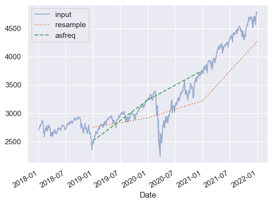
# resample() --> 데이터를 집계 --> 전년도 평균 보여줌
# asfreq() --> 데이터를 선택 --> 연말 주가 보여줌
sp500.plot(alpha=0.5, style='-')
# resampling
sp500.resample('BYE').mean().plot(style=':')
sp500.asfreq('BYE').plot(style='--');
plt.legend(['input', 'resample', 'asfreq'],
loc='upper left');
1
2
3
4
5
6
7
8
fig, ax = plt.subplots(2, sharex=True)
data = sp500.iloc[:10]

data.asfreq('D').plot(ax=ax[0], marker='o')

data.asfreq('D', method='bfill').plot(ax=ax[1], style='-o')
data.asfreq('D', method='ffill').plot(ax=ax[1], style='--o')
ax[1].legend(["back-fill", "forward-fill"]);

Time-shifts
1
2
3
4
5
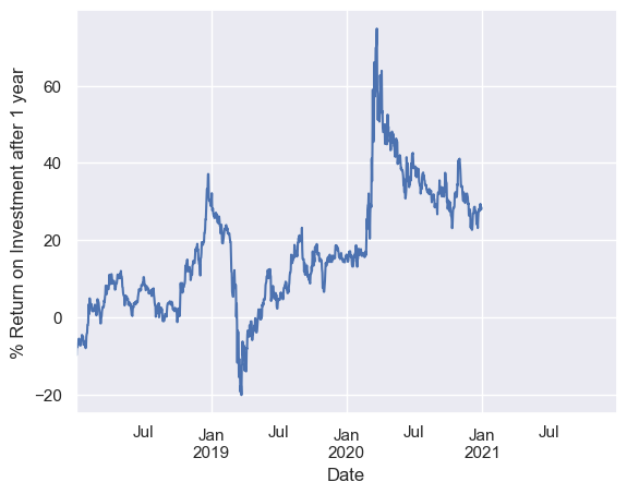
sp500 = sp500.asfreq('D', method='pad')
# 주어진 항목 수만큼 데이터를 이동하는데 shift 메서드 사용
ROI = 100 * (sp500.shift(-365) - sp500) / sp500
ROI.plot()
plt.ylabel('% Return on Investment after 1 year');
Rolling windows
1
2
3
4
5
6
7
8
9
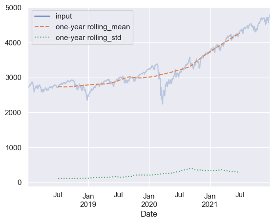
# 롤링 통계
# 인덱스의 1년 중심 롤링 평균과 표준 편차
rolling = sp500.rolling(365, center=True)
data = pd.DataFrame({'input': sp500,
'one-year rolling_mean': rolling.mean(),
'one-year rolling_std': rolling.std()})
ax = data.plot(style=['-', '--', ':'])
ax.lines[0].set_alpha(0.3)
Example: Visualizing Seattle Bicycle Counts
1
2
3
data = pd.read_csv('FremontBridge.csv', index_col='Date', parse_dates=True, date_format='%m/%d/%Y %I:%M:%S %p')
data.columns = ['Total', 'West', 'East']
data.head()
| Total | West | East | |
|---|---|---|---|
| Date | |||
| 2012-10-02 13:00:00 | 55.0 | 7.0 | 48.0 |
| 2012-10-02 14:00:00 | 130.0 | 55.0 | 75.0 |
| 2012-10-02 15:00:00 | 152.0 | 81.0 | 71.0 |
| 2012-10-02 16:00:00 | 278.0 | 167.0 | 111.0 |
| 2012-10-02 17:00:00 | 563.0 | 393.0 | 170.0 |
1
data.dropna().describe()
| Total | West | East | |
|---|---|---|---|
| count | 100735.000000 | 100735.000000 | 100735.000000 |
| mean | 105.352827 | 45.553373 | 59.799454 |
| std | 131.840748 | 60.090291 | 81.591238 |
| min | 0.000000 | 0.000000 | 0.000000 |
| 25% | 13.000000 | 5.000000 | 7.000000 |
| 50% | 59.000000 | 25.000000 | 32.000000 |
| 75% | 143.000000 | 62.000000 | 78.000000 |
| max | 1097.000000 | 667.000000 | 850.000000 |
Visualizing the data
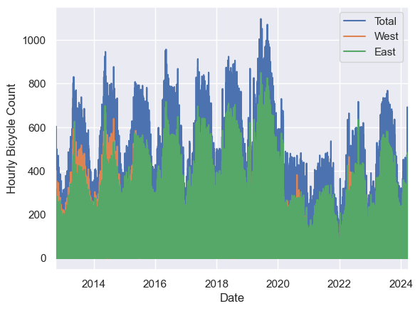
1
2
data.plot()
plt.ylabel('Hourly Bicycle Count');
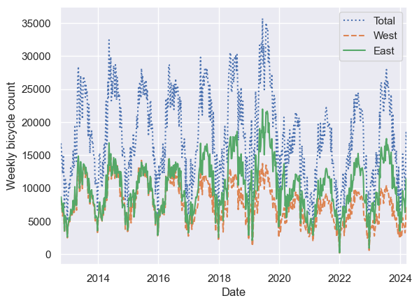
1
2
3
4
# 밀집도를 낮추기 위해 주 단위로 리샘플링
weekly = data.resample('W').sum()
weekly.plot(style=[':', '--', '-'])
plt.ylabel('Weekly bicycle count');
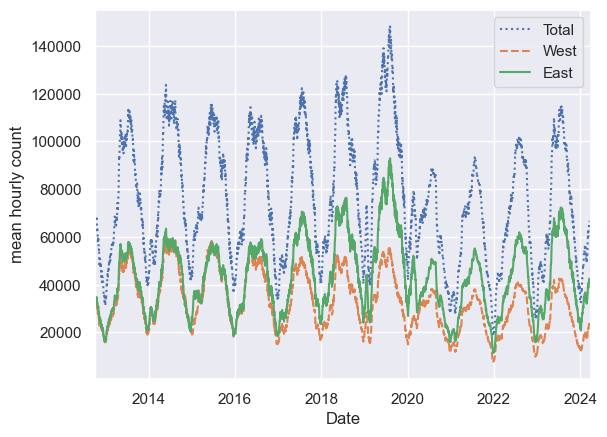
1
2
3
4
# 30일 롤링 평균을 구해 데이터가 중심에 오게 하기
daily = data.resample('D').sum()
daily.rolling(30, center=True).sum().plot(style=[':', '--', '-'])
plt.ylabel('mean hourly count');
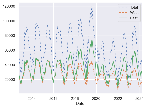
1
2
3
# 가우스 윈도우 함수 사용
daily.rolling(50, center=True,
              win_type='gaussian').sum(std=10).plot(style=[':', '--', '-']);
Digging into the data
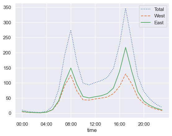
1
2
3
4
# 하루 시간대별 통행량
by_time = data.groupby(data.index.time).mean()
hourly_ticks = 4 * 60 * 60 * np.arange(6)
by_time.plot(xticks=hourly_ticks, style=[':', '--', '-']);
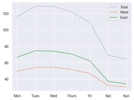
1
2
3
4
# 요일에 따른 통행량
by_weekday = data.groupby(data.index.dayofweek).mean()
by_weekday.index = ['Mon', 'Tues', 'Wed', 'Thurs', 'Fri', 'Sat', 'Sun']
by_weekday.plot(style=[':', '--', '-']);
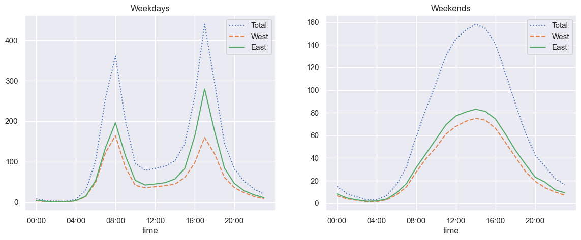
1
2
3
# 주말 표시 플래그와 시간대별 분류
weekend = np.where(data.index.weekday < 5, 'Weekday', 'Weekend')
by_time = data.groupby([weekend, data.index.time]).mean()
1
2
3
4
5
6
7
8
# 주중과 주말의 시간대별 추이
import matplotlib.pyplot as plt

fig, ax = plt.subplots(1, 2, figsize=(14, 5))
by_time.loc['Weekday'].plot(ax=ax[0], title='Weekdays',
                            xticks=hourly_ticks, style=[':', '--', '-'])
by_time.loc['Weekend'].plot(ax=ax[1], title='Weekends',
                            xticks=hourly_ticks, style=[':', '--', '-']);
이 기사는 저작권자의 CC BY-NC 4.0 라이센스를 따릅니다.