Aggregation_And_Grouping
1
2
3
4
5
6
7
8
9
10
11
12
13
14
15
16
17
18
19
20
| import numpy as np
import pandas as pd
class display(object):
"""Display HTML representation of multiple objects"""
template = """<div style="float: left; padding: 10px;">
<p style='font-family:"Courier New", Courier, monospace'>{0}</p>{1}
</div>"""
def __init__(self, *args):
self.args = args
def _repr_html_(self):
return '\n'.join(self.template.format(a, eval(a)._repr_html_())
for a in self.args)
def __repr__(self):
return '\n\n'.join(a + '\n' + repr(eval(a))
for a in self.args)
|
Planets Data
1
2
3
4
5
| # 이 데이터는 외행성 주변에서 발견한 행성에 대한 정보 제공
import seaborn as sns
planets = sns.load_dataset('planets')
planets.shape
|
| method | number | orbital_period | mass | distance | year |
|---|
| 0 | Radial Velocity | 1 | 269.300 | 7.10 | 77.40 | 2006 |
|---|
| 1 | Radial Velocity | 1 | 874.774 | 2.21 | 56.95 | 2008 |
|---|
| 2 | Radial Velocity | 1 | 763.000 | 2.60 | 19.84 | 2011 |
|---|
| 3 | Radial Velocity | 1 | 326.030 | 19.40 | 110.62 | 2007 |
|---|
| 4 | Radial Velocity | 1 | 516.220 | 10.50 | 119.47 | 2009 |
|---|
Pandas의 간단한 집계 연산 Simple Aggregation in Pandas
1
2
3
4
| # Series
rng = np.random.RandomState(42)
ser = pd.Series(rng.rand(5))
print("ser:\n", ser, "\n\nser.sum():", ser.sum(), "\n\nser.mean():", ser.mean())
|
1
2
3
4
5
6
7
8
9
10
11
| ser:
0 0.374540
1 0.950714
2 0.731994
3 0.598658
4 0.156019
dtype: float64
ser.sum(): 2.811925491708157
ser.mean(): 0.5623850983416314
|
1
2
3
4
| # DataFrame
df = pd.DataFrame({'A': rng.rand(5),
'B': rng.rand(5)})
print("df:\n", df, "\n\ndf.mean():\n", df.mean(), "\n\ndf.mean(axis='columns'):\n", df.mean(axis='columns'))
|
1
2
3
4
5
6
7
8
9
10
11
12
13
14
15
16
17
18
19
20
| df:
A B
0 0.155995 0.020584
1 0.058084 0.969910
2 0.866176 0.832443
3 0.601115 0.212339
4 0.708073 0.181825
df.mean():
A 0.477888
B 0.443420
dtype: float64
df.mean(axis='columns'):
0 0.088290
1 0.513997
2 0.849309
3 0.406727
4 0.444949
dtype: float64
|
1
2
| # describe() --> 각 열에 대한 여러 일반적인 집계를 계산하고 결과를 반환
planets.dropna().describe()
|
| number | orbital_period | mass | distance | year |
|---|
| count | 498.00000 | 498.000000 | 498.000000 | 498.000000 | 498.000000 |
|---|
| mean | 1.73494 | 835.778671 | 2.509320 | 52.068213 | 2007.377510 |
|---|
| std | 1.17572 | 1469.128259 | 3.636274 | 46.596041 | 4.167284 |
|---|
| min | 1.00000 | 1.328300 | 0.003600 | 1.350000 | 1989.000000 |
|---|
| 25% | 1.00000 | 38.272250 | 0.212500 | 24.497500 | 2005.000000 |
|---|
| 50% | 1.00000 | 357.000000 | 1.245000 | 39.940000 | 2009.000000 |
|---|
| 75% | 2.00000 | 999.600000 | 2.867500 | 59.332500 | 2011.000000 |
|---|
| max | 6.00000 | 17337.500000 | 25.000000 | 354.000000 | 2014.000000 |
|---|
Pandas의 집계 메서드 목록
| Aggregation | Description |
|---|
count() | 항목 전체 개수 Total number of items |
first(), last() | 첫 항목과 마지막 항목 First and last item |
mean(), median() | 평균값과 중앙값 Mean and median |
min(), max() | 최솟값과 최댓값 Minimum and maximum |
std(), var() | 표준편차와 분산 Standard deviation and variance |
mad() | 절대 평균 편차 Mean absolute deviation |
prod() | 전체 항목의 곱 Product of all items |
sum() | 전체 항목의 합 Sum of all items |
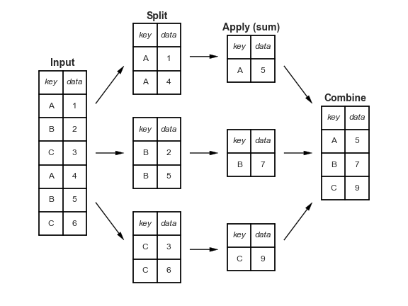
GroupBy: Split, Apply, Combine 분할, 적용, 결합
- 분할 단계: 지정된 키 값을 기준으로 DataFrame을 나누고 분류하는 단계
- 적용 단계: 개별 그룹 내에서 일반적으로 집계, 변환, 필터링 같은 함수를 계산
- 결합 단계: 이 연산의 결과를 결과 배열에 병합
1
2
3
| df = pd.DataFrame({'key': ['A', 'B', 'C', 'A', 'B', 'C'],
'data': range(6)}, columns=['key', 'data'])
df
|
| key | data |
|---|
| 0 | A | 0 |
|---|
| 1 | B | 1 |
|---|
| 2 | C | 2 |
|---|
| 3 | A | 3 |
|---|
| 4 | B | 4 |
|---|
| 5 | C | 5 |
|---|
1
2
| # 분할-적용-결합 연산 계산 --> DataFrameGroupBy 객체 리턴
df.groupby('key')
|
1
| <pandas.core.groupby.generic.DataFrameGroupBy object at 0x000001F4DCD07D70>
|
1
2
| # DataFrameGroupBy 객체에 집계 연산 적용
display("df.groupby('key').sum()", "df.groupby('key').mean()", "df.groupby('key').max()")
|
The GroupBy object
Column indexing
GroupBy 객체는 DataFrame과 동일한 방식으로 열 인덱싱을 지원하며 수정된 GroupBy 객체를 리턴
1
| planets.groupby('method')
|
1
| <pandas.core.groupby.generic.DataFrameGroupBy object at 0x000001F4DCD07800>
|
1
| planets.groupby('method')['orbital_period']
|
1
| <pandas.core.groupby.generic.SeriesGroupBy object at 0x000001F4DD0A0350>
|
1
| planets.groupby('method')['orbital_period'].median()
|
1
2
3
4
5
6
7
8
9
10
11
12
| method
Astrometry 631.180000
Eclipse Timing Variations 4343.500000
Imaging 27500.000000
Microlensing 3300.000000
Orbital Brightness Modulation 0.342887
Pulsar Timing 66.541900
Pulsation Timing Variations 1170.000000
Radial Velocity 360.200000
Transit 5.714932
Transit Timing Variations 57.011000
Name: orbital_period, dtype: float64
|
Iteration over groups
GroupBy 객체는 그룹을 직접 순회할 수 있도록 지원하며, 각 그룹을 Series나 DataFrame으로 리턴
1
2
| for (method, group) in planets.groupby('method'):
print("{0:30s} shape={1}".format(method, group.shape))
|
1
2
3
4
5
6
7
8
9
10
| Astrometry shape=(2, 6)
Eclipse Timing Variations shape=(9, 6)
Imaging shape=(38, 6)
Microlensing shape=(23, 6)
Orbital Brightness Modulation shape=(3, 6)
Pulsar Timing shape=(5, 6)
Pulsation Timing Variations shape=(1, 6)
Radial Velocity shape=(553, 6)
Transit shape=(397, 6)
Transit Timing Variations shape=(4, 6)
|
Dispatch methods
GroupBy 객체가 명시적으로 구현하지 않은 메서드는 객체에 상관없이 일부 파이썬 클래스 매직을 통해 그 그룹에 전달되고 호출
Dispatch methods는 각 개별 그룹에 적용되고 그 결과는 GroupBy 내에서 결합돼 리턴
1
| planets.groupby('method')['year'].describe().unstack()
|
1
2
3
4
5
6
7
8
9
10
11
12
13
| method
count Astrometry 2.0
Eclipse Timing Variations 9.0
Imaging 38.0
Microlensing 23.0
Orbital Brightness Modulation 3.0
...
max Pulsar Timing 2011.0
Pulsation Timing Variations 2007.0
Radial Velocity 2014.0
Transit 2014.0
Transit Timing Variations 2014.0
Length: 80, dtype: float64
|
1
2
3
4
5
6
| rng = np.random.RandomState(0)
df = pd.DataFrame({'key': ['A', 'B', 'C', 'A', 'B', 'C'],
'data1': range(6),
'data2': rng.randint(0, 10, 6)},
columns=['key', 'data1', 'data2'])
df
|
| key | data1 | data2 |
|---|
| 0 | A | 0 | 5 |
|---|
| 1 | B | 1 | 0 |
|---|
| 2 | C | 2 | 3 |
|---|
| 3 | A | 3 | 3 |
|---|
| 4 | B | 4 | 7 |
|---|
| 5 | C | 5 | 9 |
|---|
Aggregation
1
2
| # 문자열, 함수, 리스트 등을 취해 한 번에 모든 집계를 계산
df.groupby('key').aggregate(['min', 'median', 'max'])
|
| data1 | data2 |
|---|
| min | median | max | min | median | max |
|---|
| key | | | | | | |
|---|
| A | 0 | 1.5 | 3 | 3 | 4.0 | 5 |
|---|
| B | 1 | 2.5 | 4 | 0 | 3.5 | 7 |
|---|
| C | 2 | 3.5 | 5 | 3 | 6.0 | 9 |
|---|
1
2
| # 열 이름을 해당 열에 적용될 연산에 매핑하는 딕셔너리 전달
df.groupby('key').aggregate({'data1': 'min', 'data2': 'max'})
|
Filtering
filter() 함수는 그룹이 필터링을 통과하는지 아닌지를 지정하는 부울 값을 리턴
1
2
3
4
5
6
| # 그룹 속성을 기준으로 데이터를 걸러냄
def filter_func(x):
return x['data2'].std() > 4
display('df', "df.groupby('key').std()", "df.groupby('key').filter(filter_func)")
|
df
| key | data1 | data2 |
|---|
| 0 | A | 0 | 5 |
|---|
| 1 | B | 1 | 0 |
|---|
| 2 | C | 2 | 3 |
|---|
| 3 | A | 3 | 3 |
|---|
| 4 | B | 4 | 7 |
|---|
| 5 | C | 5 | 9 |
|---|
df.groupby('key').std()
| data1 | data2 |
|---|
| key | | |
|---|
| A | 2.12132 | 1.414214 |
|---|
| B | 2.12132 | 4.949747 |
|---|
| C | 2.12132 | 4.242641 |
|---|
df.groupby('key').filter(filter_func)
| key | data1 | data2 |
|---|
| 1 | B | 1 | 0 |
|---|
| 2 | C | 2 | 3 |
|---|
| 4 | B | 4 | 7 |
|---|
| 5 | C | 5 | 9 |
|---|
1
2
| # 재결합을 위해 전체 데이터의 변환된 버전을 반환 --> 결과는 입력과 같은 형상
df.groupby('key').transform(lambda x: x - x.mean())
|
| data1 | data2 |
|---|
| 0 | -1.5 | 1.0 |
|---|
| 1 | -1.5 | -3.5 |
|---|
| 2 | -1.5 | -3.0 |
|---|
| 3 | 1.5 | -1.0 |
|---|
| 4 | 1.5 | 3.5 |
|---|
| 5 | 1.5 | 3.0 |
|---|
The apply() method
임의의 함수를 그룹 결과에 적용할 때 사용
DataFrame을 취해 Pandas 객체나 스칼라를 반환
결합 연산은 반환된 출력값 유형에 따라 조정
1
2
3
4
5
6
7
8
| # 첫 번째 열을 두 번째 열의 합계로 정규화
def norm_by_data2(x):
# x is a DataFrame of group values
x['data1'] /= x['data2'].sum()
return x
display('df', "df.groupby('key').apply(norm_by_data2, include_groups=False)")
|
df
| key | data1 | data2 |
|---|
| 0 | A | 0 | 5 |
|---|
| 1 | B | 1 | 0 |
|---|
| 2 | C | 2 | 3 |
|---|
| 3 | A | 3 | 3 |
|---|
| 4 | B | 4 | 7 |
|---|
| 5 | C | 5 | 9 |
|---|
df.groupby('key').apply(norm_by_data2, include_groups=False)
| | data1 | data2 |
|---|
| key | | | |
|---|
| A | 0 | 0.000000 | 5 |
|---|
| 3 | 0.375000 | 3 |
|---|
| B | 1 | 0.142857 | 0 |
|---|
| 4 | 0.571429 | 7 |
|---|
| C | 2 | 0.166667 | 3 |
|---|
| 5 | 0.416667 | 9 |
|---|
분할 키 지정 Specifying the split key
분할 키를 제공하는 리스트, 배열, 시리즈, 인덱스 A list, array, series, or index providing the grouping keys
1
2
| L = [0, 1, 0, 1, 2, 0]
display('df', 'df.groupby(L).sum()', "df.groupby(df['key']).sum()")
|
df
| key | data1 | data2 |
|---|
| 0 | A | 0 | 5 |
|---|
| 1 | B | 1 | 0 |
|---|
| 2 | C | 2 | 3 |
|---|
| 3 | A | 3 | 3 |
|---|
| 4 | B | 4 | 7 |
|---|
| 5 | C | 5 | 9 |
|---|
df.groupby(L).sum()
| key | data1 | data2 |
|---|
| 0 | ACC | 7 | 17 |
|---|
| 1 | BA | 4 | 3 |
|---|
| 2 | B | 4 | 7 |
|---|
df.groupby(df['key']).sum()
인덱스를 그룹에 매핑한 딕셔너리나 시리즈 A dictionary or series mapping index to group
1
2
3
| df2 = df.set_index('key')
mapping = {'A': 'vowel', 'B': 'consonant', 'C': 'consonant'}
display('df2', 'df2.groupby(mapping).sum()')
|
df2
| data1 | data2 |
|---|
| key | | |
|---|
| A | 0 | 5 |
|---|
| B | 1 | 0 |
|---|
| C | 2 | 3 |
|---|
| A | 3 | 3 |
|---|
| B | 4 | 7 |
|---|
| C | 5 | 9 |
|---|
df2.groupby(mapping).sum()
| data1 | data2 |
|---|
| key | | |
|---|
| consonant | 12 | 19 |
|---|
| vowel | 3 | 8 |
|---|
Any Python function
1
| display('df2', 'df2.groupby(str.lower).mean()')
|
df2
| data1 | data2 |
|---|
| key | | |
|---|
| A | 0 | 5 |
|---|
| B | 1 | 0 |
|---|
| C | 2 | 3 |
|---|
| A | 3 | 3 |
|---|
| B | 4 | 7 |
|---|
| C | 5 | 9 |
|---|
df2.groupby(str.lower).mean()
| data1 | data2 |
|---|
| key | | |
|---|
| a | 1.5 | 4.0 |
|---|
| b | 2.5 | 3.5 |
|---|
| c | 3.5 | 6.0 |
|---|
A list of valid keys
1
| df2.groupby([str.lower, mapping]).mean()
|
| | data1 | data2 |
|---|
| key | key | | |
|---|
| a | vowel | 1.5 | 4.0 |
|---|
| b | consonant | 2.5 | 3.5 |
|---|
| c | consonant | 3.5 | 6.0 |
|---|
Grouping example
1
2
3
4
| decade = 10 * (planets['year'] // 10)
decade = decade.astype(str) + 's'
decade.name = 'decade'
planets.groupby(['method', decade])['number'].sum().unstack().fillna(0)
|
| decade | 1980s | 1990s | 2000s | 2010s |
|---|
| method | | | | |
|---|
| Astrometry | 0.0 | 0.0 | 0.0 | 2.0 |
|---|
| Eclipse Timing Variations | 0.0 | 0.0 | 5.0 | 10.0 |
|---|
| Imaging | 0.0 | 0.0 | 29.0 | 21.0 |
|---|
| Microlensing | 0.0 | 0.0 | 12.0 | 15.0 |
|---|
| Orbital Brightness Modulation | 0.0 | 0.0 | 0.0 | 5.0 |
|---|
| Pulsar Timing | 0.0 | 9.0 | 1.0 | 1.0 |
|---|
| Pulsation Timing Variations | 0.0 | 0.0 | 1.0 | 0.0 |
|---|
| Radial Velocity | 1.0 | 52.0 | 475.0 | 424.0 |
|---|
| Transit | 0.0 | 0.0 | 64.0 | 712.0 |
|---|
| Transit Timing Variations | 0.0 | 0.0 | 0.0 | 9.0 |
|---|