Sorting_Arrays

배열 정렬 Sorting Arrays

L = [3, 1, 4, 1, 5, 9, 2, 6]
L.sort()  # 정렬만 하고 반환하지 않음
print(L)
sorted('python')  # 정렬된 복사본 반환

[1, 1, 2, 3, 4, 5, 6, 9]





['h', 'n', 'o', 'p', 't', 'y']

NumPy의 빠른 정렬 Fast Sorting in NumPy

import numpy as np

x = np.array([2, 1, 4, 3, 5])
np.sort(x)  # sorted와 유사

array([1, 2, 3, 4, 5])

x = np.array([2, 1, 4, 3, 5])
i = np.argsort(x)  # sort와 유사
print(i)  # 정렬된 요소의 인덱스를 반환
x[i]

[1 0 3 2 4]





array([1, 2, 3, 4, 5])

행이나 열 기준 정렬 Sorting along rows or columns

rand = np.random.RandomState(42)
X = rand.randint(0, 10, (4, 6))
print("X:\n", X)
print("\nX의 각 열을 정렬:\n", np.sort(X, axis=0))
print("\nX의 각 행을 정렬:\n", np.sort(X, axis=1))

X:
 [[6 3 7 4 6 9]
 [2 6 7 4 3 7]
 [7 2 5 4 1 7]
 [5 1 4 0 9 5]]

X의 각 열을 정렬:
 [[2 1 4 0 1 5]
 [5 2 5 4 3 7]
 [6 3 7 4 6 7]
 [7 6 7 4 9 9]]

X의 각 행을 정렬:
 [[3 4 6 6 7 9]
 [2 3 4 6 7 7]
 [1 2 4 5 7 7]
 [0 1 4 5 5 9]]

부분정렬: 파티션 나누기 Partial Sorts: Partitioning

x = np.array([7, 2, 3, 1, 6, 5, 4])
# x 배열의 반환된 파티션 왼쪽에 가장 작은 값 세 개, 나머지 오른쪽
print("x:", x)
print("\nnp.partition(x, 3):", np.partition(x, 3))

# X 배열의 첫 두 개의 슬롯에 해당 행의 가장 작은 값 두 개
print("\nX:\n", X)
print("\nnp.partition(X, 2, axis=1):\n", np.partition(X, 2, axis=1))

x: [7 2 3 1 6 5 4]

np.partition(x, 3): [2 1 3 4 6 5 7]

X:
 [[6 3 7 4 6 9]
 [2 6 7 4 3 7]
 [7 2 5 4 1 7]
 [5 1 4 0 9 5]]

np.partition(X, 2, axis=1):
 [[3 4 6 7 6 9]
 [2 3 4 7 6 7]
 [1 2 4 5 7 7]
 [0 1 4 5 9 5]]

Example: k-최근접 이웃 알고리즘 k-Nearest Neighbors

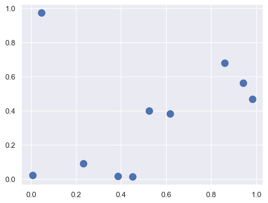
# 10x2 배열
X = rand.rand(10, 2)

# 산포도로 표시
%matplotlib
inline
import matplotlib.pyplot as plt
import seaborn;

seaborn.set()
plt.scatter(X[:, 0], X[:, 1], s=100);

# 제곱 거리 행렬 계산
dist_sq = np.sum((X[:, np.newaxis, :] - X[np.newaxis, :, :]) ** 2, axis=-1)

# 제곱 거리 행렬 계산 코드 구성
differences = X[:, np.newaxis, :] - X[np.newaxis, :, :]  # 각 쌍의 점 사이의 좌표 차이를 계산
sq_differences = differences ** 2  # 좌표 차이를 제곱
dist_sq = sq_differences.sum(-1)  # 제곱 거리를 구하기 위해 좌표 차이를 더함
dist_sq.diagonal()  # 행렬 대각선(각 점과 그 점 사이의 거리 집합)이 모두 0인지 확인

array([0., 0., 0., 0., 0., 0., 0., 0., 0., 0.])

nearest = np.argsort(dist_sq, axis=1)
print(nearest)

[[0 3 9 7 1 4 2 5 6 8]
 [1 4 7 9 3 6 8 5 0 2]
 [2 1 4 6 3 0 8 9 7 5]
 [3 9 7 0 1 4 5 8 6 2]
 [4 1 8 5 6 7 9 3 0 2]
 [5 8 6 4 1 7 9 3 2 0]
 [6 8 5 4 1 7 9 3 2 0]
 [7 9 3 1 4 0 5 8 6 2]
 [8 5 6 4 1 7 9 3 2 0]
 [9 7 3 0 1 4 5 8 6 2]]

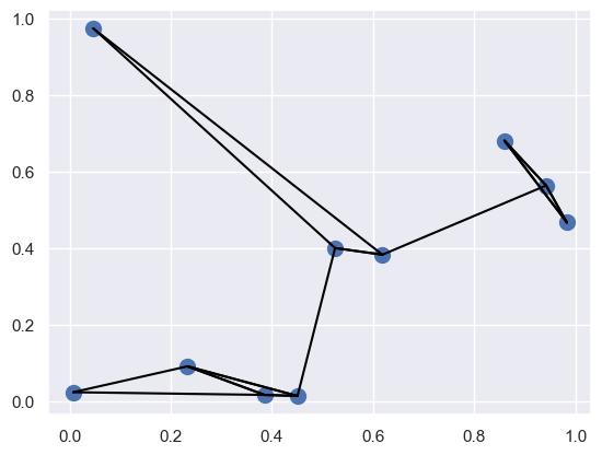
K = 2
nearest_partition = np.argpartition(dist_sq, K + 1, axis=1)

plt.scatter(X[:, 0], X[:, 1], s=100)
# 각 점을 두 개의 가장 가까운 이웃과 선으로 이음
for i in range(X.shape[0]):
    for j in nearest_partition[i, :K + 1]:
        # X[i]부터 X[j]까지 선으로 이음
        #  zip 매직 함수를 이용
        plt.plot(*zip(X[j], X[i]), color='black')